Getting started - a single particle

In this tutorial, we’ll simulate the stochastic dynamics of a single nanoparticle. We model clusters of nanoparticles using the magpy.Model class. In this case we only have a single particle in our cluster. The first step is to import magpy.

import magpy as mp

To create our model, we need to specify the geometry and material properties of the system. The units and purpose of each property is defined below.

Name	Description	Units
Radius	The radius of the spherical particle	m
Anisotropy	Magnitude of the anisotropy	J/m\(^3\)
Anisotropy axis	Unit vector indicating the direction of the anisotropy
Magnetisation	Saturation magnetisation of every particle in the cluster	A/m
Magnetisation direction	Unit vector indicating the initial direction of the magnetisation
Location	Location of the particle within the cluster	m
Damping	The damping constant of every particle in the cluster
Temperature	The ambient temperature of the cluster (fixed)	K

Note: radius, anisotropy, anisotropy_axis, magnetisation_direction, and location vary for each particle and must be specified as a list.

single_particle = mp.Model(
    radius = [12e-9],
    anisotropy = [4e4],
    anisotropy_axis = [[0., 0., 1.]],
    magnetisation_direction = [[1., 0., 0.]],
    location = [[0., 0., 0.]],
    damping = 0.1,
    temperature = 300.,
    magnetisation = 400e3
)

Simulate

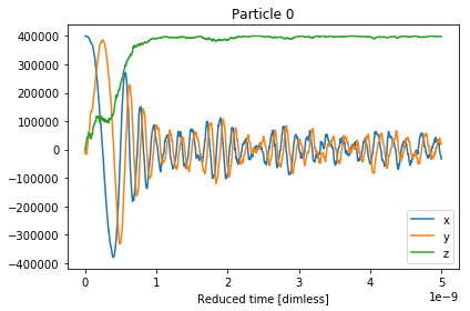
A simulation in magpy consists of simulating the magnetisation vector of the particle in time. In the model above we specified the initial magnetisation vector along the \(x\)-axis and the anisotropy along the \(z\)-axis. Since it is energetically favourable for the magnetisation to align with its anisotropy axis, we should expect the magnetisation to move toward the \(z\)-axis. With some random fluctuations.

The simulate function is called with the following parameters: - end_time the length of the simulation in seconds - time_step the time step of the integrator in seconds - max_samples in order to save memory, the output is down/upsampled as required. So if you simulate a billion steps, you can only save the state at 1000 regularly spaced intervals. - seed for reproducible simulations you should always choose the seed.

results = single_particle.simulate(
    end_time = 5e-9,
    time_step = 1e-14,
    max_samples=1000,
    seed = 1001
)

The x,y,z components of the magnetisation can be visualised with the .plot() function.

results.plot()

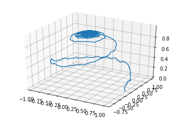
We can also access this data directly and plot it however we like! In this example, we normalise the magnetisation and plot it in 3d space.

import matplotlib.pyplot as plt
from mpl_toolkits.mplot3d import Axes3D
%matplotlib inline

Ms = 400e3
time = results.time
mx = results.x[0] / Ms # particle 0
my = results.y[0] / Ms # particle 0
mz = results.z[0] / Ms # particle 0

fg = plt.figure()
ax = fg.add_subplot(111, projection='3d')
ax.plot3D(mx, my, mz)

[<mpl_toolkits.mplot3d.art3d.Line3D at 0x7f4f95319a58>]